Example Burgers' equation

In this notebook we provide a simple example of the DeepMoD algorithm by applying it on the Burgers' equation.

We start by importing the required libraries and setting the plotting style:

# General imports
import numpy as np
import torch
import matplotlib.pylab as plt

# DeepMoD functions

from deepymod import DeepMoD
from deepymod.model.func_approx import NN
from deepymod.model.library import Library1D
from deepymod.model.constraint import LeastSquares
from deepymod.model.sparse_estimators import Threshold,PDEFIND
from deepymod.training import train
from deepymod.training.sparsity_scheduler import TrainTestPeriodic
from scipy.io import loadmat

# Settings for reproducibility
np.random.seed(42)
torch.manual_seed(0)


%load_ext autoreload
%autoreload 2

Next, we prepare the dataset.

data = np.load('data/burgers.npy', allow_pickle=True).item()
print('Shape of grid:', data['x'].shape)

Shape of grid: (256, 101)

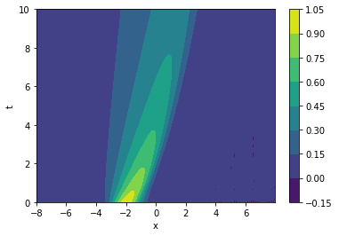
Let's plot it to get an idea of the data:

fig, ax = plt.subplots()
im = ax.contourf(data['x'], data['t'], np.real(data['u']))
ax.set_xlabel('x')
ax.set_ylabel('t')
fig.colorbar(mappable=im)

plt.show()

png

X = np.transpose((data['t'].flatten(), data['x'].flatten()))
y = np.real(data['u']).reshape((data['u'].size, 1))
print(X.shape, y.shape)

(25856, 2) (25856, 1)

As we can see, $X$ has 2 dimensions, $\{x, t\}$ , while $y$ has only one, $\{u\}$ . Always explicity set the shape (i.e. $N\times 1$ , not $N$ ) or you'll get errors. This dataset is noiseless, so let's add $2.5\%$ noise:

noise_level = 0.025
y_noisy = y + noise_level * np.std(y) * np.random.randn(y[:,0].size, 1)

The dataset is also much larger than needed, so let's hussle it and pick out a 1000 samples:

number_of_samples = 2000

idx = np.random.permutation(y.shape[0])
X_train = torch.tensor(X[idx, :][:number_of_samples], dtype=torch.float32, requires_grad=True)
y_train = torch.tensor(y_noisy[idx, :][:number_of_samples], dtype=torch.float32)

print(X_train.shape, y_train.shape)

torch.Size([2000, 2]) torch.Size([2000, 1])

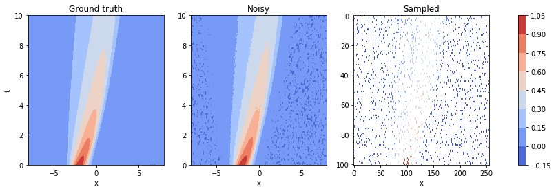
We now have a dataset which we can use. Let's plot, for a final time, the original dataset, the noisy set and the samples points:

fig, axes = plt.subplots(ncols=3, figsize=(15, 4))

im0 = axes[0].contourf(data['x'], data['t'], np.real(data['u']), cmap='coolwarm')
axes[0].set_xlabel('x')
axes[0].set_ylabel('t')
axes[0].set_title('Ground truth')

im1 = axes[1].contourf(data['x'], data['t'], y_noisy.reshape(data['x'].shape), cmap='coolwarm')
axes[1].set_xlabel('x')
axes[1].set_title('Noisy')

sampled = np.array([y_noisy[index, 0] if index in idx[:number_of_samples] else np.nan for index in np.arange(data['x'].size)])
sampled = np.rot90(sampled.reshape(data['x'].shape)) #array needs to be rotated because of imshow

im2 = axes[2].imshow(sampled, aspect='auto', cmap='coolwarm')
axes[2].set_xlabel('x')
axes[2].set_title('Sampled')

fig.colorbar(im1, ax=axes.ravel().tolist())

plt.show()

png

Configuring DeepMoD

Configuration of the function approximator: Here the first argument is the number of input and the last argument the number of output layers.

network = NN(2, [30, 30, 30, 30], 1)

Configuration of the library function: We select athe library with a 2D spatial input. Note that that the max differential order has been pre-determined here out of convinience. So, for poly_order 1 the library contains the following 12 terms: * [ $1, u_x, u_{xx}, u_{xxx}, u, u u_{x}, u u_{xx}, u u_{xxx}, u^2, u^2 u_{x}, u^2 u_{xx}, u^2 u_{xxx}$ ]

library = Library1D(poly_order=2, diff_order=3)

Configuration of the sparsity estimator and sparsity scheduler used. In this case we use the most basic threshold-based Lasso estimator and a scheduler that asseses the validation loss after a given patience. If that value is smaller than 1e-5, the algorithm is converged.

estimator = Threshold(0.1) 
sparsity_scheduler = TrainTestPeriodic(periodicity=50, patience=200, delta=1e-5)

Configuration of the sparsity estimator

constraint = LeastSquares() 
# Configuration of the sparsity scheduler

Now we instantiate the model and select the optimizer

model = DeepMoD(network, library, estimator, constraint)

# Defining optimizer
optimizer = torch.optim.Adam(model.parameters(), betas=(0.99, 0.99), amsgrad=True, lr=1e-3)

Run DeepMoD

We can now run DeepMoD using all the options we have set and the training data: * The directory where the tensorboard file is written (log_dir) * The ratio of train/test set used (split) * The maximum number of iterations performed (max_iterations) * The absolute change in L1 norm considered converged (delta) * The amount of epochs over which the absolute change in L1 norm is calculated (patience)

train(model, X_train, y_train, optimizer,sparsity_scheduler, log_dir='runs/Burgers/', split=0.8, max_iterations=100000)

 13350  MSE: 2.53e-05  Reg: 1.38e-05  L1: 1.45e+00 Algorithm converged. Writing model to disk.

Sparsity masks provide the active and non-active terms in the PDE:

model.sparsity_masks

[tensor([False, False,  True, False, False,  True, False, False, False, False,
         False, False])]

estimatior_coeffs gives the magnitude of the active terms:

print(model.estimator_coeffs())

[array([[ 0.        ],
       [ 0.        ],
       [ 0.39227325],
       [ 0.        ],
       [ 0.        ],
       [-1.001875  ],
       [ 0.        ],
       [ 0.        ],
       [ 0.        ],
       [ 0.        ],
       [ 0.        ],
       [ 0.        ]], dtype=float32)]

So the final terms that remain are the $u_{xx}$ and $u u_{x}$ resulting in the following Burgers equation (in normalized coefficients: $u_t = 0.4 u_{xx} - u u_{x}$ .